did kinney county break its desired future conditions? part deux

After my first post on this topic, a little bird tweeted in my ear [please read the following in sotto voce], “Look at the groundwater management plan! Look at the groundwater management plan!” So I did.

Wow.

I’m not sure where to start, but I will start with these tldr statements: (1) These are the most convoluted desired future conditions I’ve ever seen and (2) the groundwater model they are based on is deeply flawed.

Now for the rest of the story…

The groundwater management plan for the Kinney Country Groundwater Conservation District has a section titled “Addressing the desired future conditions” and, within this section, adds some interpretation of the district’s desired future conditions.

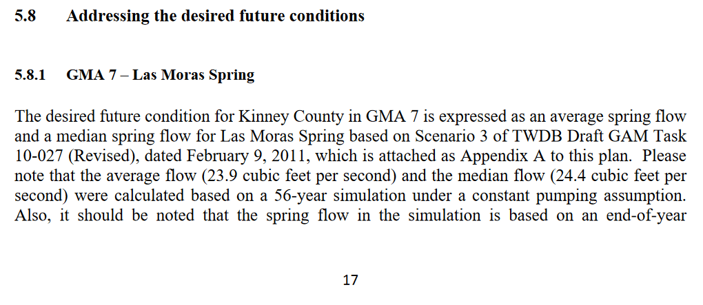
“The desired future condition for Kinney County in GMA 7 is expressed as an average spring flow and a median spring flow for Las Moras Spring based on Scenario 3 of TWDB Draft GAM Task 10-027 (Revised), dated February 9, 2011, which is attached as Appendix A to this plan.”

This is different than the official desired future conditions but provides the district’s interpretation of its conditions (or so it seems…). So, according to this, it’s all about spring flow at Las Moras Springs. Also, it appears the reference in the official desired future conditions is incorrect and should be the one listed above. Note that the numbers in this management plan refer to the older set of desired future conditions and not the most recent ones, although the difference is subtle (the average is the same but the median is slightly lower in the current desired future conditions).

Along with the clarification comes a handful of silt:

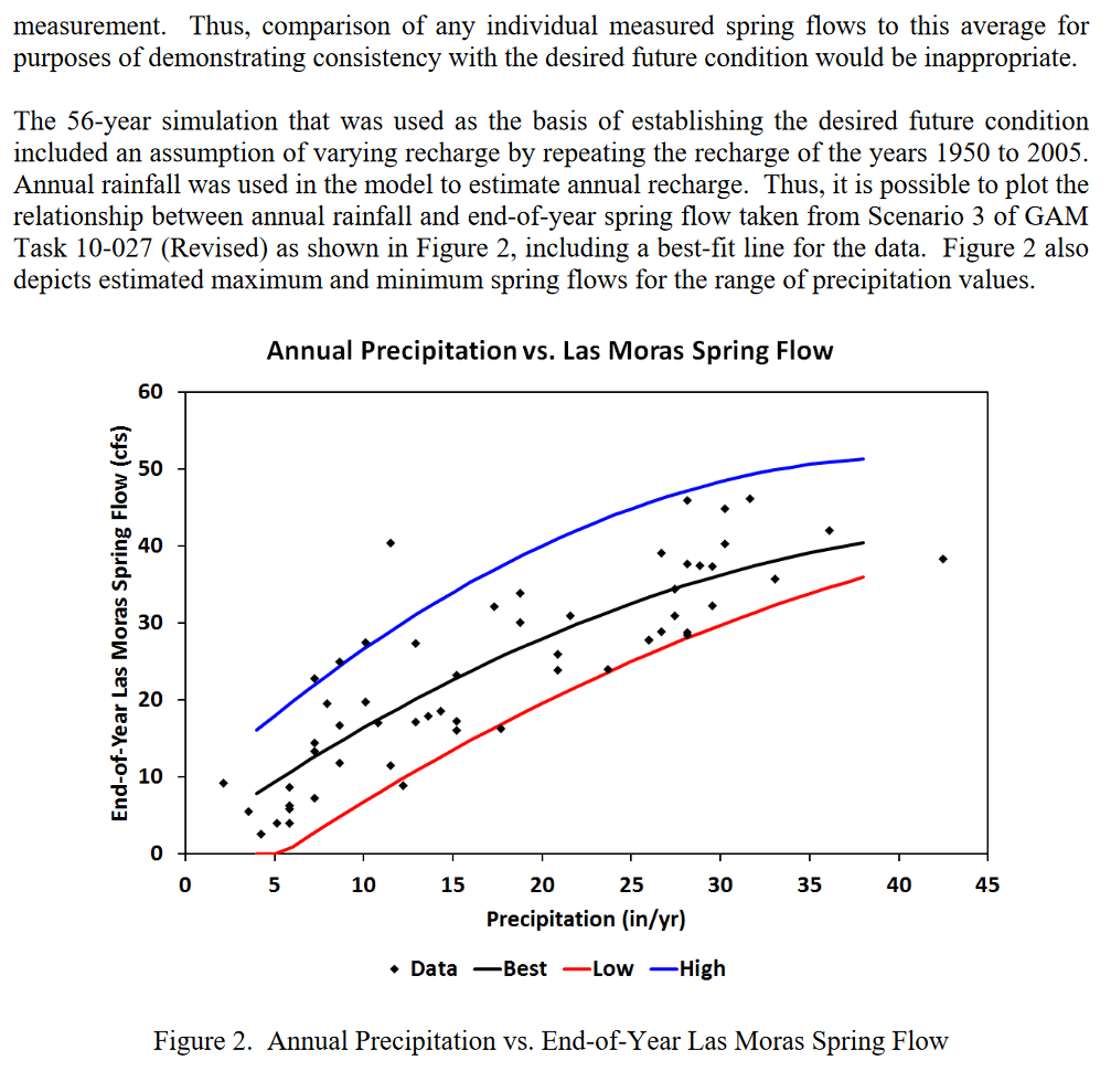
“…it should be noted that the spring flow in the simulation is based on an end-of-year measurement. Thus, comparison of any individual measured spring flows to this average for purposes of demonstrating consistency with the desired future condition would be inappropriate.”

Alright. The DFC does say “average” and “median,” which means, indeed, that any spot measurement cannot be compared the desired future condition numbers. However, I’m not sure I agree with the use of “measurement” in this statement. First off, if I wanted to be a pedantic ass on terminology, I could point out that nothing is “measured” in a model—it is simulated. But I don’t want to be a pedantic ass, so I will let that slip of the keyboard pass us by.

This end-of-the-year business is interesting. The model does spit out a springflow for the end of the stress period, where a stress period is a chunk of time in the model where “stresses” (such as pumping and other things, such as recharge and boundary conditions) remain the same. So, indeed, the model reports a springflow at the end of the stress period. However, the water that flows out of the spring is summed over the entire stress period such that is represents an average springflow for that stress period. There are things called time steps that allow a modeler to output what’s going on within a stress period, but there’s no mention of time steps in the model run not the model report.

Later, the model run states that:

“Note that because the model was run on annual stress periods, these spring flows are representative of end-of-the calendar year conditions. Thus, for comparative purposes, flows collected in December and January should be used to track with the desired future condition.”

That’s not correct if the springflows used to define the desired future conditions source from annual stress periods. Later use of model data suggests a step away from this “December and January” approach.

The average and median used in the DFC source from this plot of model output (from Appendix A of the groundwater management plan):

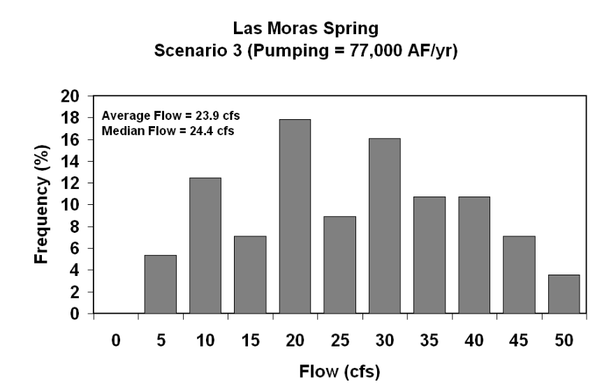
Figure 1: A histogram of simulated annual average flow from Las Moras Springs with 77,000 acre-feet per year of pumping.

There are 101 values represented here, 56 from the historical run and then a repeat of the recharge conditions from 1950 to 2005. I need to stress that these springflows are model outputs for a range of recharge conditions for a set amount of pumping of 77,000 acre-feet per year (more on this pumping later…). The average and median flows noted in the desired future conditions are based on these model outputs. OK.

But then things get a little kooky.

Section 5.8.1 of the groundwater management plan lays out how to determine whether or not the district is in compliance with the desired future conditions in Groundwater Management Area 7. I’ve provided screen captures of it at the bottom of this post for your own enjoyment.

The first thing to note from Section 5.8.1 is that the desired future conditions are not stated in a way that reflects what the actual desired future conditions are. The actual desired future conditions are not the average and median springsflows in Figure 1; the actual desired future conditions are the statistical distribution represented in Figure 1. More accurately, the desired future conditions are a kinda-sorta statistical representation of the statistical distribution in Figure 1. Got that?

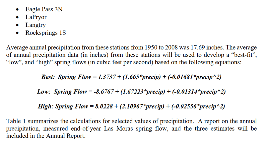
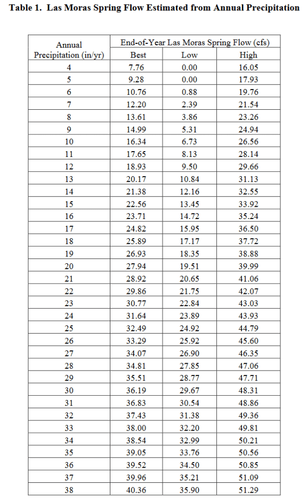
To get there, Section 5.8.1 presents a relationship between springflow and precipitation because “[a]nnual rainfall was used in the model to estimate annual recharge”:

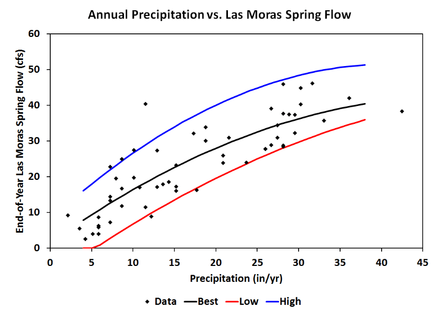
Figure 2: The relationship between annual precipitation and simulated flow at Las Moras Springs with 77,000 acre-feet per year of pumping. The lines show the best fit (black) and the estimated maximum (blue) and estimated minimum (red) flows.

The equations that describe these lines are:

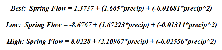
where precip is the average of the annual precipitation measured at the weather stations at Brackettville, Del Rio AP, Eagle Pass 3N, LaPryor, Langtry, and Rocksprings 1S.

So… in order to evaluate compliance with the desired future conditions, you have to analyze rainfall across the region; use the equations above to calculate the best, low, and high expected springflows (with 77,000 acre-feet per year of pumping); and compare annual average springflow to that value. Presumably, the desired future conditions are busted if springflows are too low or (oddly) too high.

So let’s see what 2024 says!

Found the data for Bracketville, Langtry, Del Rio but (oops) there is no Rocksprings 1S weather station (but there is a Rocksprings station) or Del Rio AP (but assuming this is Del Rio International Airport). There’s an Eagle Pass 3 N, but it stopped collecting data in July of 2018 (but there is a Piedras Negras OBS). There’s a La Pryor, but it stopped collecting data in August of 2021 (and there’s not a substitute). The data for Brackettville is incomplete (only 19 daily measurements for 2024) as is Del Rio Laughlin AFB (317 measurements), Piedras Negras OBS (350), and Rocksprings (295).

Maybe I’m missing something, but there is no possible way to evaluate the DFC with the stated methodology.

For grins, let’s use the data we have as a hint of where we might be. Rocksprings reported 11.86 inches in 2024, Piedras Negras reported 7.51 inches, and Del Rio Laughlin AFB reported 10.37 inches (I did not include Langtry because that station appears to have stopped measuring rainfall in 2022). That averages out to 9.9 inches (or 10 inches for gummint work). That means the average springflow for Las Moras Springs should be between 6.73 and 26.56 cubic feet per second. The average flow that I calculated was 5.9, so perhaps the desired future conditions were not met?

A side note about the model: it is deeply flawed. The model is calibrated with historical pumping levels of about 70,000 acre-feet per year. That ain’t right. Actual pumping has been around 3,000 to 5,000 acre-feet per year (with a recent foray into 10,000 acre-feet per year). So the model is calibrated with pumping that is more than 10 times higher than it should be. The springs have gone dry with with ~10,000 acre-feet per year of pumping in a severe drought. Imagine what springflows would look like with 70,000 acre-feet per year of pumping (or the 77,000 acre-feet of pumping the desired future conditions are based on).

You might say “But Robert! The model is nicely calibrated!” Why, yes—yes, it is. However, numerical models suffer from non-uniqueness if they are poorly constrained, and that is the case here. Nonuniqueness means that, with the available information, there are multiple solutions to the same problem. There is water flowing out two sides of the county, but we don’t know how much. That allows for nonuniqueness.

And there you have it, the full monte (I hope…). I offer this up as hopefully helpful to the district and, since the district is hiring a new consultant, to the new consultant, as well as to the constituents.

———————————————————-

Relevant excerpt from the groundwater management plan: